Boosting | 의사결정나무

Boosting, 의사결정나무의 초전설 최종진화형(테이블데이터 분석의 정수)

해당 포스트는 전북대학교 통계학과 최규빈 교수님의 강의내용을 토대로 재구성되었음을 알립니다.

1. 라이브러리 imports

import numpy as np
import pandas as pd
import matplotlib.pyplot as plt
import sklearn.tree
import sklearn.ensemble

#---#
import warnings
warnings.filterwarnings('ignore')
#---#
import matplotlib.animation
import IPython

2. 사용할 데이터

np.random.seed(43052)
temp = pd.read_csv('https://raw.githubusercontent.com/guebin/DV2022/master/posts/temp.csv').iloc[:,3].to_numpy()[:80]
temp.sort()
eps = np.random.randn(80)*3 # 오차
icecream_sales = 20 + temp * 2.5 + eps 
df_train = pd.DataFrame({'temp':temp,'sales':icecream_sales})
df_train

	temp	sales
0	-4.1	10.900261
1	-3.7	14.002524
2	-3.0	15.928335
3	-1.3	17.673681
4	-0.5	19.463362
...	...	...
75	9.7	50.813741
76	10.3	42.304739
77	10.6	45.662019
78	12.1	48.739157
79	12.4	46.007937

80 rows × 2 columns

아이스크림 그거 맞다.

3. 기존의 분석법 체크

- 선형

• 선형회귀
• 로지스틱회귀
• Lasso, Ridge

---

- 의사결정나무

파라미터 위주 모형의 한계를 극복

• 배깅 : 부스트랩, 다양성
• 랜덤포레스트 : 부스트랩, 약한 트리ㆍ더 큰 다양성
• 부스팅??? : 성장.

부스팅은 약한 트리가 점점 강한 트리로 성장하는 느낌이다.

4. 부스팅으로 일단 적합

## step 1
X = df_train[['temp']]
y = df_train['sales']

## step 2
predictr = sklearn.ensemble.GradientBoostingRegressor()  ## 기울기 부스팅 회귀...?

## step 3
predictr.fit(X, y)

## step 4
yhat = predictr.predict(X)

plt.plot(X, y, 'o')
plt.plot(X, yhat, '--')
plt.show()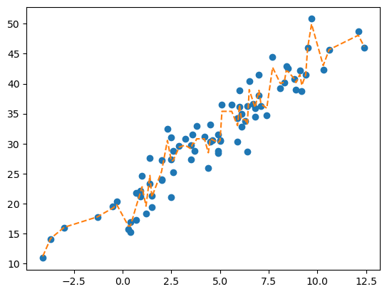

먼가 기존 트리보다 상당히 완만함.

5. yhat을 얻는 과정 : 어려움…

- my_trees 생성

predictr.estimators_[0][0]  ## 얘네는 이중 리스트를 써서 두번 인덱스를 지정해줘야 똑같음... 뭐임...

DecisionTreeRegressor(criterion='friedman_mse', max_depth=3,
                      random_state=RandomState(MT19937) at 0x13753387440)

In a Jupyter environment, please rerun this cell to show the HTML representation or trust the notebook.
On GitHub, the HTML representation is unable to render, please try loading this page with nbviewer.org.

trees = [t[0] for t in predictr.estimators_]
trees[0]

DecisionTreeRegressor(criterion='friedman_mse', max_depth=3,
                      random_state=RandomState(MT19937) at 0x13753387440)

In a Jupyter environment, please rerun this cell to show the HTML representation or trust the notebook.
On GitHub, the HTML representation is unable to render, please try loading this page with nbviewer.org.

- 단순시도 (여태껏 그랬듯이 나무들의 평균으로) – 실패

_yhat = np.array([tree.predict(X) for tree in trees]).mean(axis = 0)
_yhat

array([-1.98529568, -1.68873716, -1.50105449, -1.32748757, -1.17877814,
       -1.12461928, -1.48130074, -1.47726246, -1.47726246, -1.14576839,
       -1.14576839, -0.93324255, -0.93324255, -0.82550938, -1.14740524,
       -0.63621774, -0.63621774, -0.99552612, -0.99552612, -0.56894418,
       -0.56894418, -0.56894418, -0.05104935, -0.39699577, -0.39699577,
       -0.39699577, -0.38296042, -0.38296042, -0.16511506, -0.13001062,
       -0.18975132, -0.18975132, -0.09772732, -0.09772732, -0.02478889,
       -0.02478889, -0.25650094, -0.02421372, -0.02421372, -0.03653755,
       -0.08676362, -0.08676362, -0.08676362, -0.05359582, -0.05359582,
        0.43424239,  0.43353213,  0.19572773,  0.19572773,  0.54183429,
        0.54183429,  0.2947621 ,  0.2947621 ,  0.2947621 ,  0.21585817,
        0.21585817,  0.7964528 ,  0.59531418,  0.49763334,  0.49763334,
        0.78455561,  0.78455561,  0.55907873,  0.48574479,  1.16729012,
        0.89795288,  0.92295305,  1.11059435,  1.09672204,  0.98224138,
        0.9138514 ,  1.05038217,  0.86805699,  1.04227523,  1.49564195,
        1.89066912,  1.19912714,  1.46250802,  1.70344969,  1.51603631])

plt.plot(X, y, 'o')
plt.plot(X, yhat, '--')
plt.plot(X, _yhat, '--')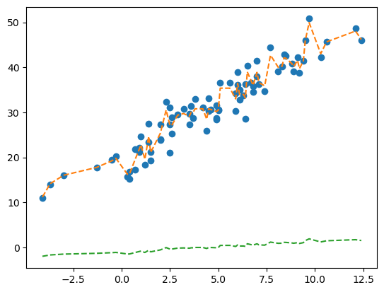

예?! 이건 아니잖아요!

plt.plot(X, y, 'o')
plt.plot(X, yhat, '--')
plt.plot(X, _yhat+y.mean(), '--')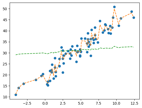

똑같잖아요!

plt.plot(X, y, 'o')
plt.plot(X, yhat, '--')
plt.plot(X, _yhat*100, '--')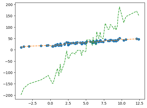

~어 근데 뭔가 윤곽선이 익숙하긴 한데…~

- 처음 3개의 의사결정나무의 예측

sklearn.tree.plot_tree(
    predictr.estimators_[0][0],
    max_depth = 1,
    feature_names = X.columns.to_list()
);

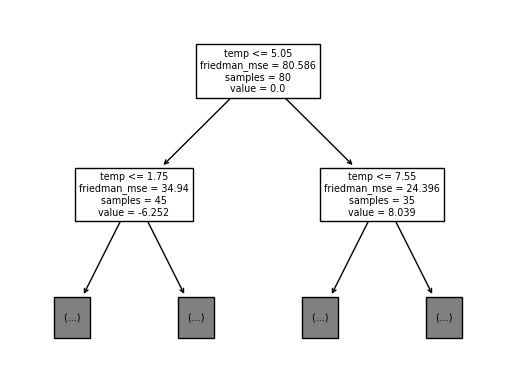
• 1번째 트리.

중심 노드를 0으로 두고, 그 양옆의 값들을 중심값에서의 차이로 설정하였음.

plt.plot(X, y, 'o')
plt.plot(X, trees[0].predict(X)+y.mean(), '--', label = 'yhat with 1st tree')
plt.plot(X, trees[1].predict(X)+y.mean(), '--', label = 'yhat with 2nd tree')
plt.plot(X, trees[2].predict(X)+y.mean(), '--', label = 'yhat with 3rd tree')
plt.plot(X, trees[-1].predict(X)+y.mean(), '--', label = 'yhat with last tree')
plt.legend()
plt.show()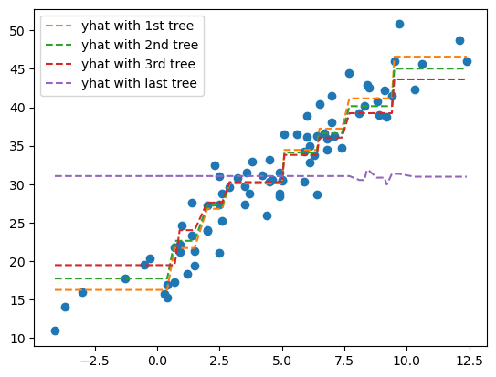

초기 값들은 어느정도 경사가 있는데, 계속 나아갈수록 직선에 가까워진다… 이걸 어떻게 합쳐야 부스팅의 예측값이 나오는 걸까???

- 시각화로 확인

• 태초 : yhat = y.mean()으로 적합
• 첫번째 나무 반영 : 현재까지의 적합값 + 첫번째 나무의 적합값 × 0.1(predictr.learning_rate) – ver 0.01
• 두번째 나무 반영 : 현재까지의 적합값 + 두번째 나무의 적합값 × 0.1 – ver 0.02

\(\dots\)

• 100번째 나무 반영 : 현재까지의 적합값 + 100번째 나무의 적합값 × 0.1 > 최종 yhat – ver 1.00

trees[0].predict(X)+trees[1].predict(X)  ## 최초 관측한 자료

array([-28.12857773, -28.12857773, -28.12857773, -28.12857773,
       -28.12857773, -28.12857773, -28.12857773, -28.12857773,
       -28.12857773, -17.76744106, -17.76744106, -17.76744106,
       -17.76744106, -17.76744106, -17.76744106, -17.76744106,
       -17.76744106, -17.76744106, -17.76744106,  -8.07411483,
        -8.07411483,  -8.07411483,  -8.07411483,  -8.07411483,
        -8.07411483,  -8.07411483,  -8.07411483,  -8.07411483,
        -1.82748008,  -1.82748008,  -1.82748008,  -1.82748008,
        -1.82748008,  -1.82748008,  -1.82748008,  -1.82748008,
        -1.82748008,  -1.82748008,  -1.82748008,  -1.82748008,
        -1.82748008,  -1.82748008,  -1.82748008,  -1.82748008,
        -1.82748008,   6.48143774,   6.48143774,   6.48143774,
         6.48143774,   6.48143774,   6.48143774,   6.48143774,
         6.48143774,   6.48143774,   6.48143774,   6.48143774,
        11.74216296,  11.74216296,  11.74216296,  11.74216296,
        11.74216296,  11.74216296,  11.74216296,  11.74216296,
        19.21655361,  19.21655361,  19.21655361,  19.21655361,
        19.21655361,  19.21655361,  19.21655361,  19.21655361,
        19.21655361,  19.21655361,  29.52785838,  29.52785838,
        29.52785838,  29.52785838,  29.52785838,  29.52785838])

predictions = [tree.predict(X) for tree in trees]  ## 각 예측값 할당

plt.plot(X, y, 'o')
plt.plot(X, np.repeat(y.mean(), len(X)), '--', label = 'WeakPredictor (ver 0.00)')
plt.plot(X,
         np.array(predictions[:1]).sum(axis = 0)*0.1 + y.mean(),
         '--', label = 'WeakPredictor (ver 0.01)')
plt.plot(X,
         np.array(predictions[:2]).sum(axis = 0)*0.1 + y.mean(),
         '--', label = 'WeakPredictor (ver 0.02)')
plt.plot(X,
         np.array(predictions[:3]).sum(axis = 0)*0.1 + y.mean(),
         '--', label = 'WeakPredictor (ver 0.03)')
plt.plot(X,
         np.array(predictions).sum(axis = 0)*0.1 + y.mean(),
         '--', label = 'WeakPredictor (ver 1.00)')
plt.legend()
plt.show()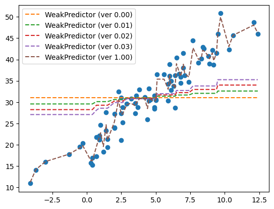

##이걸로 해도 되기는 하는데, 이건 항상 predict()를 해줘야하니까 연산이 반복되서 리소스 할당에 좋지 않을듯
##np.array([trees[i].predict(X) for i in range(2)]).mean(axis = 0)

- 해당 과정을 애니메이션으로 표현

## 어셈블리 코드
def ensemble(trees, i = None) :
    if i is None :
        i = len(trees)
    else :
        i = i+1  ## loc하게 되면 그것 다음것까지로 넣어야되니까.
    yhat = np.array(predictions[:i]).sum(axis = 0)*0.1 + y.mean()  ## 축의 값들을 가중치를 반영하여 더해야 함.
    return yhat

fig, ax = plt.subplots(1)
plt.close()  ## 쌩 피규어가 콘솔에 안뜨도록 함.

def func(frame) :
    ax.clear()
    ax.plot(X, y, 'o', label = 'RawData')  ## 원자료
    ax.plot(X, ensemble(trees, frame), '--', label = 'WeakPredictor (ver ({})'.format(round((frame+1)*0.01, 3)))
    ax.legend()

ani = matplotlib.animation.FuncAnimation(fig, func, frames = 100)

display(IPython.display.HTML(ani.to_jshtml()))

Once Loop Reflect

6. 재현

애초에 그러면 각각의 트리를 어떻게 적합한거지?

A. 재현의 확인

---

- 아이디어 :

• 처음부터 yhat을 강하게 학습하지 않고 약하게 조금씩 학습하다.
• 부족한 공부는 (학습이 덜 되어있는 부분 : SSE = y - yhat)은 조금씩 강화하면서 보완하자.

- 구현 : my_trees, my_residuals를 직접 구현

trees[0]

DecisionTreeRegressor(criterion='friedman_mse', max_depth=3,
                      random_state=RandomState(MT19937) at 0x13753387440)

In a Jupyter environment, please rerun this cell to show the HTML representation or trust the notebook.
On GitHub, the HTML representation is unable to render, please try loading this page with nbviewer.org.

my_trees = []
my_residuals = []

res = y - y.mean()  ## 잔차(태초의)

## 100번 공부
for i in range(100) :
    tree = sklearn.tree.DecisionTreeRegressor(max_depth = 3, criterion = 'friedman_mse')
    tree.fit(X, res)  ## 아직 적합되지 못한 잔차에 대해서 적합을 함(오버피팅???)
    yhat = tree.predict(X)
    res = res - yhat*0.1  ## 학습한 것을 다 반영하지 말고 learning_rate만큼만 반영하자.
    my_trees.append(tree)
    my_residuals.append(res)

## 덜 깊게 적합하는 선에서 잔차를 적합하고, 또 적합하고... 이 과정을 100번 반복한다.

- 비교 : my_trees와 trees의 비교(고정된 i)

i = 10
fig = plt.figure()
ax = fig.subplots(2,2)
plt.close()

ax[0,0].plot(X, y, 'o', alpha = 0.5)
ax[0,0].plot(X, ensemble(trees, i), '--')
ax[0,0].set_title('Boosting yhat')

ax[0,1].plot(X, y, 'o', alpha = 0.5)
ax[0,1].plot(X, ensemble(my_trees, i), '--')
ax[0,1].set_title('Handmade yhat')

sklearn.tree.plot_tree(trees[i], max_depth = 0, ax = ax[1,0], feature_names = X.columns.to_list())
sklearn.tree.plot_tree(my_trees[i], max_depth = 0, ax = ax[1,1], feature_names = X.columns.to_list())

fig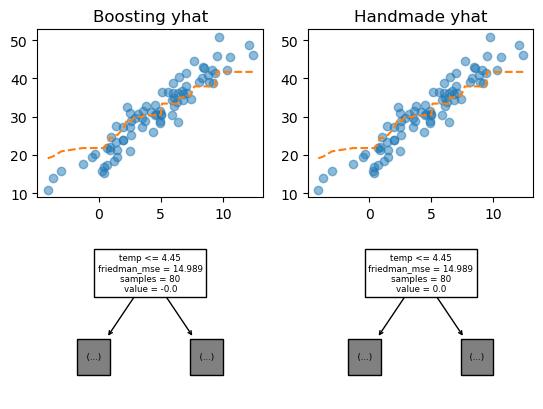

모두 일치하는 것을 알 수 있다. 잘 구현함

- 비교 : 애니메이션

## ax가 2차원 개체가 for문을 직접 걸어줄 수 음슴.

fig, ax = plt.subplots(2,2)
plt.close()

def func(frame) :
    for i in range(2) :
        for j in range(2) :
            ax[i,j].clear()
            ax[i,j].plot(X, y, 'o', alpha = 0.5)

    ax[0,0].plot(X, ensemble(trees, frame), '--')
    ax[0,1].plot(X, ensemble(my_trees, frame), '--')

    sklearn.tree.plot_tree(trees[frame], max_depth = 0, feature_names = X.columns.to_list(), ax = ax[1,0])
    sklearn.tree.plot_tree(my_trees[frame], max_depth = 0, feature_names = X.columns.to_list(), ax = ax[1,1])

ani = matplotlib.animation.FuncAnimation(fig, func, frames = 100)

display(IPython.display.HTML(ani.to_jshtml()))

Once Loop Reflect

두 결과가 완전히 동일하다. 따라서 랜덤포레스트의 트리별 동작은 위의 코드와 같다고 볼 수 있다.

### B. Step별 분석

fig, ax = plt.subplots(1,4, figsize = (10, 3))
plt.close()

def func(frame) :
    for a in ax :
        a.clear()

    ax[0].set_title('Step 0')
    ax[0].plot(X, y, 'o', alpha = 0.5)
    ax[0].plot(X, ensemble(my_trees, frame), '--')
    
    ax[1].set_title('Step 1 : Residuals')  ## 적합하고 남은 잔차를 계산
    ax[1].plot(X, my_residuals[frame], 'o', alpha = 0.5)  ## 잔차 시각화
    ax[1].set_ylim(-20,20)
    
    ax[2].set_title('Step 2 : Fitting')  ## 잔차에 대해 트리로 적합
    ax[2].plot(X, my_residuals[frame], 'o', alpha = 0.5)
    ax[2].plot(X, my_trees[frame].predict(X), '--')  ## 잔차에 대한 적합선
    ax[2].set_ylim(-20,20)
    
    ax[3].set_title('Step 3 : Update')
    ax[3].plot(X, y, 'o', alpha = 0.5)
    ax[3].plot(X, ensemble(my_trees, frame), '--', color = 'C1')
    ax[3].plot(X, ensemble(my_trees, frame+1), '--', color = 'C3')

ani = matplotlib.animation.FuncAnimation(fig, func, frames = 100)

display(IPython.display.HTML(ani.to_jshtml()))

Once Loop Reflect

- Step 0

• 파란점 y : 원래 공부할 양
• 주황색 선분 yhat : 현재까지 공부한 양

- Step 1

• i번째 남아있는 공부량(residuals)

- Step 2

• i번째 남아있는 공부량에 대해 트리로 적합(덜 빡빡하게 적합함. max_depth = 3)
• 적합을 진행할 수록 분기점이 달라짐(나중에 되면 바깥 영역으로도 적합함)

- Step 3

• 적합한 뒤 새로 갱신된 내용, 이 크기는 업데이트가 될 수록 줄어듦.

#

• 관찰1 : “Step1 : Residuals”은 점점 단순오차처럼 변화한다.(잔차에 선형성이 있었다가 정규분포처럼 모임)
• 관찰2 : “Step2 : Fitting”의 분기점들은 고정된 값이 아니다.(계속 변화한다.)
• 관찰3 : “Step3 : Update” 업데이트 되는 양은 반복이 진행될 수록 점점 작아진다.

- 느낌 : 조금씩 데이터를 학습한다.(남아있는 공부량에 대해서…) 학습할 자료가 오차항처럼 보인다면? 그때는 적합을 멈춘다.(오버피팅 방지, 피팅하면 직선이 되니까 알고리즘이 자동으로 멈춥니당. 물론 샘플을 뽑는 과정에서 계속해서 오버피팅을 시도하긴 함.)

트리의 수를 굳이 100개 꽉 채우지 말고 중간에서 끊어도 되잖아?